
University of Vermont University of Vermont
UVM ScholarWorks UVM ScholarWorks
College of Engineering and Mathematical
Sciences Faculty Publications
College of Engineering and Mathematical
Sciences
1-1-2020
A tandem evolutionary algorithm for identifying causal rules from A tandem evolutionary algorithm for identifying causal rules from
complex data complex data
John P. Hanley
University of Vermont
Donna M. Rizzo
University of Vermont
Jeffrey S. Buzas
University of Vermont
Margaret J. Eppstein
University of Vermont
Follow this and additional works at: https://scholarworks.uvm.edu/cemsfac
Part of the Human Ecology Commons, and the Medicine and Health Commons
Recommended Citation Recommended Citation
Hanley JP, Rizzo DM, Buzas JS, Eppstein MJ. A tandem evolutionary algorithm for identifying causal rules
from complex data. Evolutionary Computation. 2020 Mar;28(1):87-114.
This Article is brought to you for free and open access by the College of Engineering and Mathematical Sciences at
UVM ScholarWorks. It has been accepted for inclusion in College of Engineering and Mathematical Sciences
Faculty Publications by an authorized administrator of UVM ScholarWorks. For more information, please contact

A Tandem Evolutionary Algorithm for
Identifying Causal Rules from Complex Data
Department of Civil and Environmental Engineering, University of Vermont,
Burlington, 05405, USA
Department of Mathematics and Statistics, University of Vermont,
Burlington, 05405, USA
Department of Computer Science, University of Vermont, Burlington, 05405, USA
https://doi.org/10.1162/evco_a_00252
Abstract
We propose a new evolutionary approach for discovering causal rules in complex clas-
sication problems from batch data. Key aspects include (a) the use of a hypergeometric
probability mass function as a principled statistic for assessing tness that quanties
the probability that the observed association between a given clause and target class is
due to chance, taking into account the size of the dataset, the amount of missing data,
and the distribution of outcome categories, (b) tandem age-layered evolutionary algo-
rithms for evolving parsimonious archives of conjunctive clauses, and disjunctions of
these conjunctions, each of which have probabilistically signicant associations with
outcome classes, and (c) separate archive bins for clauses of different orders, with dy-
namically adjusted order-specic thresholds. The method is validated on majority-on
and multiplexer benchmark problems exhibiting various combinations of heterogene-
ity, epistasis, overlap, noise in class associations, missing data, extraneous features, and
imbalanced classes. We also validate on a more realistic synthetic genome dataset with
heterogeneity, epistasis, extraneous features, and noise. In all synthetic epistatic bench-
marks, we consistently recover the true causal rule sets used to generate the data. Fi-
nally, we discuss an application to a complex real-world survey dataset designed to
inform possible ecohealth interventions for Chagas disease.
Keywords
Evolutionary algorithm, epistasis, heterogeneity, multiplexer, learning classier sys-
tems, machine learning.
1 Introduction
The causal rules underlying emergent properties of complex systems often exhibit het-
erogeneity, epistasis, and/or overlap. Empirical observations of such systems may be
high-dimensional and typically include missing data, noise, and imbalanced classes.
All of these complicate our ability to infer meaningful rule sets that map observed sys-
tem features to outcomes of interest. We do not just seek “black box” association models
with high prediction accuracy on a particular data sample. Rather, our primary intent
is to develop a practical method for identifying parsimonious “white box,” potentially
Manuscript received: 13 June 2018; revised: 10 January 2019; accepted: 1 February 2019.
© 2019 Massachusetts Institute of Technology Evolutionary Computation 28(1): 87–114
J. P. Hanley et al.
causal, rule sets from data with these complexities. We aim to show that we can consis-
tently recover the causal rule sets used to generate data samples in several benchmark
problems with these complex characteristics. Succeeding in this task will increase con-
dence that we can identify potentially causal rule sets on messy real-world complex
datasets. Such rule sets will not only provide robust prediction accuracy over different
samples of the data, but importantly may also provide meaningful insights into causa-
tion, and thus inform interventions that could potentially change outcomes.
Heterogeneity exists when there are multiple underlying causes for the same out-
come class. Evidence for heterogeneity exists in many systems, including bladder cancer
(Urbanowicz et al., 2013), autism (Buxbaum et al., 2001), and American political parties
(Poole and Rosenthal, 1984). Epistasis occurs when combinations of different feature
values exhibit non-additive effects on outcomes, and is believed to be ubiquitous for
many diseases (Moore, 2003), including breast cancer (Ritchie et al., 2001), blood pres-
sure in rats (Rapp et al., 1998), and Behçet’s disease (Kirino et al., 2013). Many systems
exhibit both heterogeneity and epistasis. For example, different (i.e., heterogeneous)
combinations of nonlinearly interacting (i.e., epistatic) transmission line outages (the
features) can cause cascading failures that lead to the same patterns of power loss in the
electrical grid (the outcome) (Eppstein and Hines, 2012). Similarly, the ecological niche
of the American black bear (Ursus americanus) is epistatic, in that the species requires
both a secluded area for denning and specic combinations of spring, summer, and au-
tumn food sources (Larivière, 2001), and heterogeneous, because of the widely different
combinations of denning and three-season diets that accommodate the bear population,
contributing to a vast geographic range that spans from southern Mexico to northern
Canada (Larivière, 2001). Furthermore, real-world datasets often include correlated fea-
tures having signicant overlap in heterogeneous explanatory rules, highly imbalanced
classes (i.e., outcome classes that appear in different frequencies in the dataset), uncer-
tainty (noise) in measured outcomes, and missing data (Hanley, 2017).
There are many practical applications that require an understanding of such com-
plex relationships, such as the development of personalized drug therapies (Wilson,
2009), predicting consumer behaviors (Young Kim and Kim, 2004), identifying gene-
gene and gene-environment causes for disease (Moore, 2003), and developing eco-
interventions to reduce disease transmission in developing countries (Hanley, 2017).
However, while the size and complexity of available datasets have recently exploded,
computational tools for analyzing such systems have not kept pace (Wu et al., 2014).
Traditional statistical, data mining, and machine learning methods, such as anal-
ysis of variance (Wilson et al., 2017; Youse et al., 2016), logistic regression (Jarlenski
et al., 2016; Li et al., 2016; Nesheli et al., 2016), and decision trees (Markellos et al.,
2016; Nesheli et al., 2016) are well suited for univariate analysis of additive models.
Some studies perform feature selection using univariate logistic regression models and
then test higher-order interactions between the selected features (Kaplinski et al., 2015;
Molina et al., 2015; Olivera et al., 2015). However, since these techniques rely on the
presence of detectable univariate signals, they are not well-suited for epistatic prob-
lems where main effects are small or non-existent. For example, when using random
forests (Breiman, 2001) with 10-fold cross-validation on the epistatic and heterogeneous
synthetic genome dataset described in Section 3.3, we found that prediction accuracy
averaged only about 55% for individual decision trees, but increased with the number of
trees in the forest (plateauing at about 69% with 500 trees, which is slightly higher than
the prediction accuracy of the true causal rule set, implying overtting); we were unable
to recover any decision trees with the true causal rules. State-of-the-art classiers using
deep learning neural networks can also yield excellent class predictions from complex
88
Evolutionary Computation Volume 28, Number 1
A Tandem EA for Identifying Causal Rules
datasets (LeCun et al., 2015), but do not attempt to produce parsimonious causal rule
sets.
Learning classier systems (LCSs) are evolutionary algorithms (EAs) originally de-
signed for real-time data assimilation in dynamically changing environments (Holland
and Reitman, 1978), but have also been employed to analyze batch classication prob-
lems with epistatic, heterogeneous and/or overlapping rules (Urbanowicz and Moore,
2009). The most common type of LCS is the Michigan-style LCS, rst introduced by
Holland and Reitman (1978), which uses a genetic algorithm to evolve a population of
classiers (conjunctive clauses that each predict an outcome). Prediction is typically
evaluated based on a weighted combination of all classiers in the population, and
tness is based (at least in part) on the number of times a classier correctly predicts
the outcome of an input feature vector (Wilson, 1995). Michigan-style LCSs can be in-
efcient and subject to bias (based on sampling order) when applied to batch data.
Pittsburgh-style LCSs, rst introduced by Smith (1980), have also been applied to batch
data by dividing the dataset into subsets, although it was reported that this dataset
division can become problematic when a niche associated with an outcome is small
(Franco et al., 2012). A Pittsburgh-style LCS evolves sets of classiers as complete solu-
tions (equivalent to disjunctions of conjunctive clauses).
After unsuccessful attempts to mine a real-world complex survey dataset on Chagas
vector infestation (described in Subsection 3.5) using the Michigan-style LCS ExSTraCS
1.0 LCS (Urbanowicz et al., 2014), we introduced a new evolutionary approach to nd
heterogeneous and epistatic associations between input features and multiple outcome
classes in large datasets (Hanley et al., 2016). In the current work, we further develop
the method, show that it efciently identies the true causal rule sets in benchmark
problems, and discuss application of the method in seeking potentially causal rule sets
in messy real-world survey data, with important practical implications.
Our approach uses two EAs in tandem, each using an age-layered population struc-
ture (Hornby, 2006), and assesses tness using a hypergeometric probability mass func-
tion (Kendall, 1952) that accounts for the size of the dataset, the amount of missing
data, and the distribution of outcome categories. The rst EA evolves an archive of
conjunctive clauses (CCs) that have a high probability of a statistically signicant as-
sociation with a given outcome. The second EA evolves disjunctions of these archived
CCs to create a parsimonious archive of probabilistically signicant clauses in disjunc-
tive normal form (DNF). See Appendix A in the Supplemental Materials (https://www
.mitpressjournals.org/doi/suppl/10.1162/evco_a_00252) for a brief discussion of dif-
ferences between the current method and the method as originally presented in Hanley
et al. (2016). Despite a similarity in names, our method is unrelated to the tandem evo-
lutionary algorithm presented in Huang et al. (2007).
This article is organized as follows. In Section 2, we present our evolutionary ap-
proach and, in Section 3, we describe the test problems used. In Section 4, we show how
the method efciently nds the true causal models in the benchmark problems tested
and show some results of the method on a complex real-world dataset related to Cha-
gas disease infestation. We discuss our ndings and compare them to published LCS
results in Section 5 and summarize our contributions in Section 6.
2 Proposed Evolutionary Algorithm
We propose a system of two EAs in tandem, capable of mining large, heterogeneous
datasets of N feature vectors for possibly epistatic and heterogeneous associations be-
tween combinations of L nominal, ordinal, and/or real-valued features that are possibly
Evolutionary Computation Volume 28, Number 1 89

J. P. Hanley et al.
predictive of a given target class outcome k. The tandem algorithm decomposes the
problem into rst (a) evolving good conjunctive clauses and (b) subsequently evolving
good disjunctions of these conjunctive clauses. This problem decomposition dramati-
cally reduces the size of the search space, as will be shown in Section 4.
The rst EA (dubbed CCEA) evolves conjunctive clauses (CCs) of various orders,
where the order is the number of features included in the clause; 1
st
-order clauses cor-
respond to main (i.e., univariate) effects. The second EA (dubbed DNFEA) combines
archived CCs with disjunctions to evolve clauses in disjunctive normal form (DNFs)
of various orders, where the order is the number of CCs in a heterogeneous rule set;
1
st
-order DNFs comprise a single CC. The CCEA and DNFEA are run separately for
each desired outcome class k to identify a causal rule set.
Both the CCEA and the DNFEA are implemented using a customized version of
the Age-Layered Population Structure (ALPS) algorithm (Hornby, 2006), as shown in
Algorithm 1. Restricting competition by segregating into sub-populations by age, and
periodically introducing new individuals into the lowest age layer, has been shown to be
effective in preventing premature convergence (Hornby, 2006). In this study, we used 5
linearly-spaced nonarchive age-layers with an age gap of 3 between layers. In the CCEA,
we maintain a maximum subpopulation of layersize = L individuals; in the DNFEA we
use layersize = 20. In both the CCEA and the DNFEA, we maintain an additional 6th
layer that serves as a parsimonious archive of probabilistically signicant conjunctive
clauses.
Pseudo code for the basic evolutionary algorithm (which is common to both the
CCEA and DNFEA) is shown in Algorithm 1, and the tandem CCEA-DNFEA system
is depicted graphically in Figure 1. We detail the tness function in Subsection 2.1,
the population model and high-level algorithm (common to both the CCEA and the
DNFEA) in Subsection 2.2, and the genetic representations and variational operators
(specic to the CCEA or DNFEA) in Subsection 2.3. Open source MATLAB code is avail-
able online (Hanley, 2019).
2.1 Fitness Function
For a given outcome class k, we dene the Fitness of a given clause using a hypergeo-
metric probability mass function (PMF) (Kendall, 1952), as follows:
Fitness(clause,k) =
N
k
N
match,k
N
tot
− N
k
N
match
− N
match,k
N
tot
N
match
, (1)
where clause is a given CC (in the CCEA) or DNF (in the DNFEA); N
k
= the total number
of input feature vectors associated with the target outcome class k (e.g., presence or
absence of a disease) without any missing values for any features present in the clause;
N
match,k
= the number of input feature vectors for which the given clause is true and
that have the target class k; N
tot
= the total number of input feature vectors without any
missing values for any features present in the clause (regardless of the output class); and
N
match
= the number of input feature vectors for which the clause is true (regardless of
class).
Equation (1) is a powerful measure of tness, since it quanties the probability that
the observed association between the clause and the target class k is due to chance, taking
into account the size of the dataset, the amount of missing data, and the distribution of
outcome categories. We seek clauses with small values for Equation (1), because lower
90
Evolutionary Computation Volume 28, Number 1
A Tandem EA for Identifying Causal Rules
Fitness values are indicative of greater probability of association between a clause and
a target class.
2.2 Population Model
2.2.1 Initialization and Aging
Initially, the population of clauses is empty. But as individuals are added, it is struc-
tured into subpopulations referred to as age layers, as a means of maintaining diversity
Evolutionary Computation Volume 28, Number 1 91
J. P. Hanley et al.
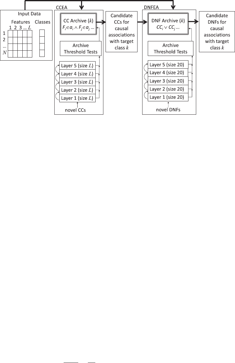
Figure 1: Graphical depiction of the proposed tandem ALPS-based EAs. For each target
class k, we use the CCEA to evolve an archive of conjunctive clauses (CCs) that pass the
threshold tests for archiving. The DNFEA then evolves disjunctions of these archived
CCs and archives clauses in disjunctive normal form (DNFs) that pass the threshold
tests for archiving.
(Hornby, 2006), with an age gap of 3 between layers. This means that every third gen-
eration, individuals in (non-empty) population layers 1–4 replace those in layers 2–5
(Alg. 1, lines 5–8) and a new random sub-population is created for layer 1, with the age
of each novel clause initialized to 0 (Alg. 1, line 9). Further details of the initialization
of CCs and DNFs are described in Subsections 2.3.1 and 2.3.2, respectively. Those aging
out of layer 5 are discarded from the population.
2.2.2 Reproduction
During each generation, all individuals in layers 1–5, plus the layersize × 5 youngest
individuals from layer 6 (the archive), are allowed to be parents (Alg. 1, lines 12–15).
Each parent produces exactly one child through either mutation or crossover, with equal
probability (Alg. 1, lines 17–29). If the child is to be produced by crossover, a second par-
ent is selected from the same or preceding (if one exists) age layer, using tournament
selection with replacement and a tournament size of 3. Details of the crossover and mu-
tation operators on CCs and DNFs are described in Subsections 2.3.1 and 2.3.2, respec-
tively. Each generation, the age of every individual that acted as a parent is incremented
by 1, and each child is given the age of its oldest parent (as in Hornby (2006)).
2.2.3 Child Placement
Every time a new clause is created, one of three things occur (Alg. 1, lines 31–37): (a) it
is discarded, (b) it is added to the archive, or (c) it is added to the population layer of
its oldest parent. Note: These steps are also carried out when new random children are
created for layer 1 (Alg. 1, line 9). Three tests determine which of these events occurs:
• Ratio Test: If (
N
mat ch,k
N
mat ch
<
N
k
N
tot
), then the clause fails the ratio test.
92
Evolutionary Computation Volume 28, Number 1

A Tandem EA for Identifying Causal Rules
• Fitness Threshold Test: If Fitness(clause,k) ≤ T
i
, where T
i
is a dynamically ad-
justed order-specic tness threshold for clauses of order i, then the clause
passes the tness threshold test.
• Optional Feature Sensitivity Threshold Test (CCs only): If Sensitivity(CC,k)
≤ S
i
, where S
i
is a dynamically adjusted order-specic sensitivity threshold for
clauses of order i, then the clause passes the feature sensitivity threshold test.
Sensitivity(CC,k) is dened as:
Sensitivity(CC,k) = max
∀F
i
∈CC
log
10
Fitness(CC,k)
Fitness(CC − F
i
,k)
, (2)
where F
i
is a feature in the CC,andCC − F
i
represents the clause with that
feature removed. Thus, Equation (2) calculates the maximum order of magni-
tude difference between the tness of a given CC and the same CC with any
one of its features removed (i.e., a lower-order, more general CC).
If a clause fails the ratio test, it is immediately discarded; this biases the algorithm
toward retaining clauses that are useful in nding associations with the target class
k. Otherwise if a DNF passes the tness threshold test, or if a CC passes both the t-
ness threshold test and the optional feature sensitivity threshold test, then the clause
is placed directly into the archive bin for order i (unless a duplicate clause is already
present). Using the additional feature sensitivity threshold test helps prevent archiving
CCs with unnecessary features (i.e., overtting the data) and also dramatically reduces
the number of archived CCs and the consequent size of the DNFEA search space. The
feature sensitivity threshold test is not used in the DNFEA, since the DNFEA only com-
bines archived CCs that have already passed this test. If a retained clause is not archived
and its oldest parent was not from the archive, it is inserted into the same population
age-layer as its oldest parent, otherwise it is discarded.
2.2.4 Archive Bins and Threshold Initialization
Each archive is partitioned into bins for different clause orders i to ensure diversity
in the complexity of archived clauses. The maximum order and bounds on bin size
are dataset-dependent (Tables C3–C5). The highest order bin may accept clauses with
order ≥ i.
All clauses in an archive bin for order i have Fitness(clause,k) ≤ T
i
(for both CCEA
and DNFEA) and optionally also Sensitivity(CC,k) ≤ S
i
(CCEA only). Thresholds T
i
,for
all orders i, are initialized to 1/N . This translates to an initial probability of 1 in N that
a clause with Fitness = T
i
is randomly associated with the target class k. In the CCEA,
S
i
is similarly initialized to log
10
(1/N ). These thresholds are dynamically reduced at the
end of each generation (Subsection 2.2.5), so that the quality of the archived clauses
increases as the evolution progresses.
2.2.5 Survivor Selection and Dynamic Threshold Adjustment
After reproduction, both nonarchive layers and archive bins may exceed their maxi-
mum allowed sizes, since new children have been added to the parent subpopulations.
When this occurs, we use truncation selection to return the overowing bins back to
their minimum allowed sizes.
For each archive bin in both the CCEA and DNFEA, the tness thresholds T
i
are
dynamically reduced to the maximum Fitness value of all clauses remaining in bin i.
If the feature sensitivity test is being used, we similarly reduce the feature sensitivity
thresholds S
i
to the maximum value of Sensitivity, over all CCs remaining in bin i.
Evolutionary Computation Volume 28, Number 1 93
J. P. Hanley et al.
2.3 Representation of Clauses
In this section, we describe the genetic representation of clauses and their variational
operators, which are specic to the CCEA (Subsection 2.3.1) and the DNFEA (Subsection
2.3.2).
2.3.1 Representation of Conjunctive Clauses (CCs)
We represent possibly epistatic interactions that are predictive of a target class k,with
CCs in the following form:
CC
k
:= F
i
∈ a
i
∧ F
j
∈ a
j
..., (3)
where := means “is dened as,” F
i
represents a feature that may be nominal, ordinal, or
continuous, and whose value lies in a
i
,and∧ represents conjunction (i.e., logical AND).
Note: a
i
is a set of values that is a proper nonempty subset of a prespecied universal
set or maximum range of each feature in the dataset. The meaning of such a clause is
interpreted as “if CC
k
is true for a given input feature vector, then the class outcome is
predicted to be k.”
Any LCS classier can be equivalently represented using the notation shown in
Equation (3). For example, the LCS classier 0##1# ⇒ 1 (where # is a wild card symbol,
which matches any value) is interpreted as “if feature 1 has value 0 and feature 4 has
value 1, then the outcome class is predicted to be 1.” The condition 0##1# is thus equiv-
alent to the conjunctive clause F
1
∈{0}∧F
4
∈{1} that is associated with outcome class
1. However, the notation in Equation (3) is more general, in that each feature F
i
can be
of any data type, and a
i
can represent any set of values of that type.
Each CC is represented by two parallel data structures. The rst is a Boolean vector
of length L, where L is the number of features in each input vector, that encodes pres-
ence (1) or absence (0) of each possible feature F
i
in the clause. Thus, the sum of the
Boolean vector represents the order of the CC and each feature i may appear at most
once in a CC. When a feature is absent from a clause, it is equivalent to the LCS nota-
tion of having a wild card in that feature’s position. We store the corresponding sets of
values a
i
in a parallel data structure, as done in De Jong and Spears (1991). This is rep-
resented as a vector of L pointers to binary masks indicating presence/absence of each
value occurring for that feature anywhere in the entire dataset. If the data are ordinal
or real-valued, we enforce all features indicated as present to have a contiguous range.
Although this approach requires space proportional to the number of unique constants
in the dataset, it affords constant-time checking to see if a given CC matches a given
instance in the dataset. These parallel structures comprise the genome of an individ-
ual in the CCEA; the values in the binary vectors representing the presence/absence of
feature F
i
, and presence/absence of values in the corresponding set a
i
, are coevolved.
We enforce at least one feature be present in each CC, and that the allowable set of
values for each included feature be non-empty; this precludes the problem, discussed
in Llorà et al. (2005), of evolving clauses that cannot match any instances in the dataset.
We allow CCs to have up to L features present, since we do not wish to make arbitrary a
priori assumptions on the maximum order of epistatic interactions that may exist and be-
cause, as shown in Iqbal et al. (2015), higher-order CCs can be useful in nding epistatic
lower-order CCs.
2.3.1.1 CC Initialization. Novel CCs are randomly created for layer 1 to guarantee
they match at least one input feature vector associated with the target class k, a process
known as “covering” (Aguilar-Ruiz et al., 2003; Bacardit and Krasnogor, 2006, 2009;
94
Evolutionary Computation Volume 28, Number 1
A Tandem EA for Identifying Causal Rules
Franco et al., 2012). To accomplish this, we rst generate a uniformly distributed ran-
dom integer j ∈{1,...,L} to specify the order of the CC, and then extract the subset
of input feature vectors with class k having at least this many nonmissing values. From
this subset, we choose one at random. While the archive is empty, this random input
feature vector is selected according to a uniform distribution. But once the archive has
been populated with clauses, we use a nonuniform distribution to bias the selection
toward input feature vectors not yet well-covered in the archive. Specically, we rst
tally the archived clauses that match each input feature vector in the extracted subset.
We then sum this tally, add one, subtract each feature vector’s tally from this value, and
cube the result (cubing increases the probability that under-represented input feature
vectors will be selected). We normalize the resulting vector and treat this as the prob-
ability distribution, then select j of the nonmissing features from the selected feature
vector to be present in the new clause according to this distribution. For each selected
feature i, we initialize a
i
to contain only the value for feature i that occurs in the selected
input feature vector.
2.3.1.2 CC Mutation. When a CC is selected for mutation, we do the following. Each
position in a copy of the binary feature array from the parent is selected with probability
1/L (if zero features were initially selected, we select one at random). For each feature
i selected, if the value at position i in the binary feature array is 0 (feature is not present
in the clause), then it is set to 1 (feature is added to the clause); and a
i
is randomly
initialized to a nonempty set (for nominal features) or contiguous range (for ordinal
or real-valued features) of allowable values that does not include the entire allowable
subset or range of values. However, if the value at position i in the binary feature array
is 1 (i.e., F
i
was present in the clause), then with probability P
w
, the bit is ipped to 0 (i.e.,
the feature is removed from the clause). We selected a high P
w
= 0.75 so mutation favors
order reduction and helps evolve parsimonious clauses with as few features as possible.
If the value at position i in the binary feature array remains a 1 (feature F
i
is still present),
the corresponding a
i
is mutated as follows. If F
i
is nominal, we randomly change, add,
or delete a categorical value to a
i
, ensuring the set remains non-empty and less than the
allowable universal set of values. If F
i
is ordinal or continuous, we randomly change
the lower or upper bound of a
i
, ensuring the range remains non-empty, contiguous, and
less than the maximum allowable range.
2.3.1.3 CC Crossover. When a CC is selected for crossover, we perform uniform
crossover between copies of the CC and a mate selected as described in Subsection 2.2.2,
where mate selection is based on Fitness. Specically, we initially create two children,
swapping values between random positions in the binary feature arrays of the two par-
ent copies, and between the same positions in the corresponding value sets/ranges. If
the rst child contains at least one feature, we discard the second child; otherwise, we
discard the rst child.
2.3.2 Representation of Clauses in Disjunctive Normal Form (DNFs)
We represent possibly heterogeneous interactions that are predictive of a target class k
with DNFs in the following form:
DNF
k
:= CC
i
∨ CC
j
..., (4)
where each CC
i
is of the form shown in Equation (3) and ∨ represents disjunction
(i.e., logical OR). The meaning of such a clause is interpreted as “if DNF
k
is true for a
given input feature vector, then the outcome class is predicted to be k.” Each DNF is
Evolutionary Computation Volume 28, Number 1 95
J. P. Hanley et al.
represented by a binary array of length N
CC,k
, where N
CC,k
is the number of CCs
archived by the CCEA for outcome class k. The binary values encode presence (1) or
absence (0) of a given CC in the DNF, so the sum of this array represents the order of
the DNF. Each DNF is constrained to include at least one CC but may have up to N
CC,k
CCs. This binary array comprises the genome of an individual in the DNFEA. For imple-
mentation efciency, prior to running the DFNEA, each CC in the archive is associated
with a precomputed binary array of length N that encodes whether the CC matches
(1) or doesn’t match (0) each of the N input feature vectors and its associated outcome
class, similar to the approach in Bacardit and Krasnogor (2006, 2009). In general, imple-
mentation of the DNFEA operators is simpler than that of the CCEA operators, since
we no longer need to worry about allowable sets/ranges or covering of input feature
vectors.
2.3.2.1 DNF Initialization. To create new DNFs for layer 1, novel DNFs are randomly
created with anywhere from one CC to the maximum DNF order that will be archived
for a given problem. If there are no DNFs in the archive, CCs are selected according to
a uniform distribution. However, if there is at least one archived DNF, then CCs are se-
lected by increasing the probability that a CC that covers more underrepresented input
feature vectors with outcome class k are selected for the initial DNF. We rst follow the
same steps described in Subsection 2.3.1.1 to create a probability distribution for select-
ing individual input feature vectors. We then create a vector with one element for each
archived CC, where each element contains the sum of the probabilities of all input fea-
ture vectors covered by one archived CC. We normalize the resulting vector and treat
this as the probability distribution for selecting a CC.
2.3.2.2 DNF Mutation. When a DNF is selected for mutation, it will undergo one of
ve mutation types with equal probability. Type 1 mutation is simple bit ip, where
each position in a copy of the binary feature array from parent
1
selected with probabil-
ity 1/N
CC,k
(if zero features were initially selected, we select one at random). We then
perform bit-ip mutation at each of these selected positions, subject to the constraint
that the DNF must still contain at least one CC.
The other four types of mutation are designed to expand the diversity of evolved
clauses in terms of PPV and coverage, or are aimed at reducing the DNF order. Type 2
mutation adds the CC that covers the most target feature vectors not covered by parent
1
(i.e., most likely to increase class coverage). Type 3 mutation adds the CC that covers
the most target feature vectors not covered by parent
1
while minimizing the number
of new non-target feature vectors covered (i.e., will most likely improve Fitness). Type
4 mutation removes the CC that covers the least target feature vectors not covered by
other CCs in the DNF (i.e., makes the DNF more parsimonious by sacricing the small-
est amount of class coverage). Finally, Type 5 mutation removes the CC that covers the
most non-target feature vectors not covered by other CCs in the DNF (i.e., makes the
DNF more parsimonious and also tries to increase the PPV). All ve mutation types
ensure that at least one CC will be present in the DNF.
2.3.2.3 DNF Crossover. When a DNF is selected for crossover, a mate is selected as
described in Subsection 2.2.2, where mate selection is based on one of four criteria (used
with equal probability): Type 1 selection picks the mate with the best Fitness.Type2se-
lection picks the mate that covers the most target feature vectors not covered by parent
1
(i.e., most likely to increase class coverage). Type 3 selection picks the mate that covers
the most target feature vectors not covered by parent
1
while minimizing the number
96
Evolutionary Computation Volume 28, Number 1

A Tandem EA for Identifying Causal Rules
Table 1: Challenges associated with benchmark problems used for testing; Majority-On
(MO), Multiplexer (MP), 4 MP variants, synthetic Genome problem, and Chagas survey
dataset.
Heter. Epistatic Overlap. Extran. Imbal. Noisy Missing
Problem Rules Rules Rules Features Classes Classes Data
MO X X
MP X X
MP V1 X X X
MP V2 X X X X
MP V3 X X X X
MP V4 X X X X
Genome X X X X X
Chagas X X X X X X X
of new nontarget feature vectors covered (i.e., will most likely improve the Fitness);
and Type 4 picks the mate with the minimum nontarget feature vectors not covered by
parent
1
(i.e., will most likely increase the PPV).
When a DNF is selected for crossover, we perform uniform or union crossover, with
equal probability. For uniform crossover, if the rst child contains at least one feature,
we discard the second child; otherwise, we discard the rst child. For union crossover,
the child is created as the union of all CCs present in either parent.
3 Test Problems
The tandem CCEA and DNFEA were explicitly designed to search for parsimonious
potentially causal rule sets in real-world problems that include heterogeneity, epistasis,
overlap, and other complexities. However, in order to increase condence on real-world
applications, we tested the efcacy of an algorithm on benchmark problems with known
causal rule sets. Unfortunately, few available benchmark problems exist in the litera-
ture with tunable heterogeneity, epistasis, and overlap, making it challenging to test
the sensitivity of the algorithm to each of these features. While others have used k-DNF
functions as benchmarks that include heterogeneity, epistasis, and overlap (Bacardit
and Krasnogor, 2009; Franco et al., 2012; Calian and Bacardit, 2013), the random way in
which these problems are generated does not allow systematic control on the degree of
overlap or class imbalance. After spending signicant time trying to generate custom
benchmark problems (e.g., Hanley et al., 2016), we appreciate the difculty in design-
ing appropriate tunable benchmarks. Consequently, in this study we test the algorithm
on three benchmarks previously used to test LCS algorithms. Two of these are classic
scalable Boolean benchmark problems (the majority-on and multiplexer problems) and
the third is a more realistic synthetic genome association problem (see Table 1). Finally,
we apply our method to a real-world Chagas survey dataset.
In the majority-on problem (Subsection 3.1), individual features do not have unique
meanings, unlike features in real-world classication problems. Yet despite known lim-
itations (McDermott et al., 2012), we include some test results on this benchmark prob-
lem because it has maximum overlap that scales with the problem size and has been
widely used as a challenging benchmark for Michigan-style LCS approaches (Iqbal
et al., 2013b,c, 2014).
Evolutionary Computation Volume 28, Number 1 97
J. P. Hanley et al.
The multiplexer problem (Subsection 3.2) is a standard benchmark problem that has
tunable heterogeneity and epistasis, although no overlap; we created 4 additional mul-
tiplexer variants that include extraneous features, varying degrees of class imbalance,
noise in class outcomes, and missing data (Table 1).
The majority-on and multiplexer problems help demonstrate how our proposed al-
gorithm can recover the exact true causal rule sets under various degrees of controllable
overlap, heterogeneity, and epistasis. We opted not to test on higher-order majority-on
or multiplexer problems, or on the hybrid-parity multiplexer function from Butz et al.
(2006), because the expected coverage of each of the individual true CCs in these prob-
lems is under 1.6%, which is less than the heuristic 5% minimum coverage proposed in
Bacardit and Krasnogor (2006) to prevent overtting and certainly less than one would
trust in an evolved solution to any real-world problem.
The synthetic genome problem (Subsection 3.3) was specically designed to ap-
proximate a more realistic dataset that contains heterogeneity, epistasis, overlapping
rules, extraneous features, and noise (Urbanowicz and Moore, 2010a).
An analysis of the entire CCEA search space evaluated on samples of input data
for the majority-on, multiplexer, and synthetic genome problems (see Appendix B in
the Supplemental Materials) illustrates (a) that there are many suboptimal clauses with
PPV greater than or equal to the PPV of the true causal clauses (and in some cases greater
coverage, as well), which underscores why PPV and coverage can be problematic t-
ness metrics for discovering the true causal CCs, (b) that the best Fitness varies between
different orders of CCs for each given problem, which is why it is important to main-
tain order-specic thresholds for the Fitness bins in the CCEA and DNFEA archives,
and (c) interesting fundamental differences in the structure of the tness landscapes of
the Boolean benchmark problems as compared to that of the more realistic synthetic
genome problem (Fig. B1).
Finally, we apply the tandem evolutionary approach to the dataset that originally
motivated the development of our algorithms. This messy real-world survey dataset
was designed to identify features most associated with the infestation of Triatoma dimidi-
ata, the vector that transmits the deadly Chagas disease, and includes correlated fea-
tures, potentially extraneous features, imbalanced classes, noise in class labels, and
missing data; previous research showed evidence that the causes of infestation are het-
erogeneous (Bustamante Zamora et al., 2015) and the root causes for infestation are sus-
pected to be inherently epistatic. This Chagas dataset (described further in Subsection
3.5) thus includes many complexities (Table 1).
Each of these test problems is dened in more detail below.
3.1 The Majority-On Problem
In the majority-on problem, the number of input features L is always odd and the out-
come class is specied by which of the Boolean values (0 or 1) is in the majority in a
particular input feature vector. The causal rule set is the set of all classiers with order
(L + 1)/2 (see Table 2), such that all xed bits and the action bit have the same value.
For example, in the 3-bit majority-on problem, the causal rule set for outcome class 0 is
the following disjunction: (00#) ∨ (0#0) ∨ (#00).
Since each condition may be considered a conjunctive clause (CC) (see Section
1), the causal rule sets may be considered in disjunctive normal form (DNF). Note:
The causal rule sets are heterogeneous (since each is the disjunction of 3 classiers).
The classiers are overlapping, yet not epistatic (i.e., all features have additive main
effects).
98
Evolutionary Computation Volume 28, Number 1

A Tandem EA for Identifying Causal Rules
Table 2: Majority-On (MO) benchmark problem characteristics. The rightmost columns
show expected change in class coverage and PPV when moving from a CC that is too
general (e.g., 1##) to the true higher-order CC that species one more feature (e.g., 11#).
Order of Order of E[Coverage] E[ Coverage] E[PPV]
Problem True CCs True DNF (per True CC) (per ↑CC Order) (per ↑CC Order)
3-bit MO 2 6 50.0% − 25.0% 25.0%
5-bit MO 3 20 25.0% − 18.8% 12.5%
7-bit MO 4 70 12.5% − 10.9% 6.3%
9-bit MO 5 252 6.3% − 5.9% 3.1%
11-bit MO 6 924 3.1% − 3.0% 1.6%
As the number of bits in the majority-on problem increases, the number of CCs in
the true causal DNF increases exponentially (Table 2). For example, in the 11-bit prob-
lem there are 924 order-6 CCs in the true causal DNF. This explosion in rule set size oc-
curs because the sensitivity of individual features drops dramatically as the majority-on
problem size increases. For example, in the 3-bit problem, adding a single feature to an
overly general CC (e.g., 1##) to turn it into a true causal CC (e.g., 11#) reduces the class
coverage by 25% but increases the PPV by 25%. However, in the 11-bit problem, mov-
ing from an overly general CC (e.g., 11111######) to a true causal CC (e.g., 111111#####)
reduces class coverage by 3% but only increases the PPV by 1.6%. Since the expected
change in PPV (Table 2, rightmost column) due to the addition of a nal true feature
drops more rapidly than the expected class coverage (Table 2, second-to rightmost col-
umn), as a function of problem size, use of a feature sensitivity test for majority-on
problems with more than 3-bits will necessarily fail. Consequently, we did not employ
the optional feature sensitivity test in solving the majority-on problems.
3.2 The Multiplexer Problem
The multiplexer problem, designed to predict the output of an electronic multiplexer
circuit, is another scalable Boolean benchmark problem. The multiplexer problem was
rst introduced to the machine learning community by Barto (1985), and has been a
standard benchmark problem for testing LCS approaches for decades (Wilson, 1987a,b;
Booker, 1989; Goldberg, 1989; De Jong and Spears, 1991; Butz et al., 2003, 2004, 2005;
Bacardit and Krasnogor, 2006; Llorà et al., 2008; Bacardit and Krasnogor, 2009; Bacardit
et al., 2009; Franco et al., 2011; Ioannides et al., 2011; Calian and Bacardit, 2013; Iqbal
et al., 2012, 2013a,b,c, 2014, 2015; Urbanowicz and Moore, 2015).
The causal rule set is the disjunction of 2
b+1
classiers, each with order b + 1, where
b is the total number of address bits used to identify a location in a vector of 2
b
data
bits that contains the outcome class. An example of the 6-bit multiplexer architecture is
presented in Table C1 (see Appendix C in the Supplemental Materials). When using the
multiplexer as a benchmark classier problem, the input feature vectors comprise both
the address bits and the data bits, so are b + 2
b
bits long; the outcome classes associated
with particular input feature vectors are thus only discovered as the address bits of the
classiers evolve. The causal rule set for outcome class 0 in the 6-bit multiplexer may
thus be considered as the following DNF: (000###) ∨ (01#0##) ∨ (10##0#) ∨ (11###0).
This benchmark problem is purely epistatic (address features do not have main effects)
Evolutionary Computation Volume 28, Number 1 99

J. P. Hanley et al.
Table 3: Multiplexer (MP) benchmark problem characteristics, where E is the expecta-
tion operator. The rightmost columns indicate the expected change in class coverage
and PPV when moving from a CC that is too general (e.g., 0#1###) to the true higher-
order CC that species one more feature (e.g., 001###).
Order of Order of E[Coverage] E[ Coverage] E[PPV]
Problem True CCs True DNF (per True CC) (per ↑Order) (per ↑Order)
6-bit MP 3 8 25.0% − 12.5% 25%
11-bit MP 4 16 12.5% − 6.3% 25%
20-bit MP 5 32 6.3% − 3.1% 25%
37-bit MP 6 64 3.1% − 1.6% 25%
and heterogeneous (different classiers match different subsets of the possible input
vectors).
In the multiplexer problem, the number of CCs in the true causal DNF increases
only linearly with the number of the problem bits (see Table 3). However, although the
expected class coverage of a given true CC, and the expected change in class cover-
age as the nal true feature is added to a CC, are both halved as the number of bits in
the problem is approximately doubled, we observe that the expected increase in PPV
due to the addition of the nal true feature remains constant at 25%, regardless of prob-
lem size (Table 3). Thus, the feature sensitivity test is able to detect important features
in the multiplexer problem.
We also report results for 4 variants of the 6-bit multiplexer problem with 14 extra-
neous features (with random binary values) added; (a) “Base Case”: balanced classes,
no noise in the output classes, and no missing data, (b) “Imbalanced”: 85% class 0 and
15% class 1, (c) “Noisy”: 20% noise in class outcomes (i.e., we ipped the outcome bit
in 20% of random input data samples), and (d) “Missing data”: 20% missing feature
values (i.e., we randomly removed 20% of feature values from the input data samples).
3.3 Synthetic Genome Problem
Urbanowicz and Moore (2010a) designed a noisy dataset to represent a synthetic
genome association study for a complex disease that incorporates both genetic epista-
sis and heterogeneity. For the remainder of this article, we refer to this as the synthetic
genome problem. The dataset contains 1,600 input feature vectors, and is perfectly bal-
anced in that 800 input feature vectors are associated with class 1 (disease) and 800 are
associated with class 0 (no disease). Each input feature vector contains 20 ternary fea-
tures, each representing whether a particular locus in the genome is homozygous for
the major allele, heterozygous, or homozygous for the minor allele.
The dataset was designed with the intent that only four of these features would
have a statistically meaningful association with the disease. Specically, there were four
heterogeneous causes for the simulated disease, in two pairs of purely epistatic inter-
actions (i.e., no main effects) between two different pairs of loci (see Table 4). Since the
association between each of these 4 causal rules and class 1 (disease) was designed to
be noisy, we also indicate their PPV, coverage, and Fitness (Table 4).
Due to noise, the true causal DNF for class 1 (i.e., the disjunction of the 4 true causal
rules shown in Table 4) has an overall PPV for class 1 of only 64% (see Table C2), cover-
age of 76%, and Fitness of 3.2 × 10
−44
.
100
Evolutionary Computation Volume 28, Number 1

A Tandem EA for Identifying Causal Rules
Table 4: The four causal rules designed to have a statistically meaningful association
with class 1 (disease) in the synthetic genome problem. In each of the 4 rules, only two
loci ∈{F
1
,F
2
,F
3
,F
4
} out of 20 are not wild cards. PPV, coverage, and Fitness of each of
these true causal rules for disease are also shown.
F
1
F
2
F
3
F
4
F
5
... F
20
N
match
N
match,k
PPV Cov. Fitness
0 1###... # 306 219 72% 27% 1.1 × 10
−17
1 0###... # 251 185 74% 23% 5.7 × 10
−17
# #01#... # 334 222 66% 28% 4.2 × 10
−12
# #10#... # 242 171 71% 21% 8.7 × 10
−13
3.4 Experimental Design for Benchmark Tests
Control parameters for the different problem types and sizes tested are shown in Ap-
pendix Tables C3–C5, for the majority-on, multiplexer, and synthetic SNP problems, re-
spectively. We note that, while preliminary experimentation showed these parameters
were sufcient for identifying the true causal clauses, it is likely they could be further
optimized to improve performance.
For the majority-on problem, the CCEA did not employ the feature sensitivity
threshold, due to the pathological nature of this problem (described in Subsection 3.1);
and we only report results for the DNFEA on the 3-bit and 5-bit majority-on problems.
This is because, without a feature sensitivity threshold in the CCEA, the CC archive for
the larger problems contained many archived CCs with orders greater than the order of
the true CCs, and there was almost no difference between the PPV of the true CCs and
those with higher order (i.e., those CCs that overt the data).
In each of the benchmark problems, the 2 outcome classes are mutually exclusive;
thus, we evolve rule sets to predict class 1, and make the assumption that ”if class 1 is
not predicted, then predict class 0,” as in Bacardit et al. (2009); Bacardit and Krasnogor
(2009); Franco et al. (2012). Runs were terminated when all of the true causal clauses
had been archived; we recorded the total number of tness evaluations performed per
run. Each problem was run for 30 random repetitions. The number of random training
input feature vectors for the majority-on and multiplexer problems was dependent on
the problem size (Tables C3–C4). The synthetic genome problem was trained on the
1,600 input feature vectors provided by Urbanowicz and Moore (2010a).
3.5 Chagas Vector Infestation Dataset
Through a collaborative effort between the University of Vermont, Loyola University
New Orleans, and La Universidad de San Carlos Guatemala, we performed detailed
socioeconomic and entomological surveys on over 20 towns in Guatemala, El Salvador,
and Honduras to study the risk of infestation with T. dimidiata, the vector for the deadly
Chagas disease (Hanley, 2017). The surveys contain 64 risk factors that experts believe
may be associated with infestation of households. Seven of the risk factors are ordinal,
six are integer, 1 is continuous, and the remaining 50 are nominal. The dataset comprises
311 input feature vectors of length 64, has 26% missing data, and imbalanced class out-
comes with 100 (32%) infested households. Because of the large number of features, we
selected relatively large CC archive bins (250 to 260 CCs per order). Since we are inter-
ested in lower-order DNFs in this application, we restricted the DNF archive to order
10 or less (100 to 110 DNFs per order).
Evolutionary Computation Volume 28, Number 1 101

J. P. Hanley et al.
Table 5: Summary of Majority-On results with no feature sensitivity test. Values repre-
sent the median over 30 repetitions.
Majority-On 3-bit 5-bit 7-bit 9-bit 11-bit
CCEA Space
1
52 484 4,372 39,364 354,292
#CCEA Evals
2
34 323 1,974 11,924 97,700
#Archived CCs
3
9 42 147 585 5,745
DNFEA Space
4
372 1.7 × 10
10
NA NA NA
#DNFEA Evals
5
255 278,818 NA NA NA
#Archived DNFs
6
53 164 NA NA NA
#Total Evals
7
294 279,307 NA NA NA
De novo DNF Space
8
2.9 × 10
6
3.1 × 10
23
NA NA NA
1
Maximum number of CCs from all possible features.
2
Median number of CCEA tness evaluations.
3
Number of CCs in the CCEA archive searched by the DNFEA.
4
Maximum number of DNFs from median number of archived CCs.
5
Median number of DNFEA tness evaluations.
6
Median number of DNFs in the DNFEA archive.
7
#CCEA Evals + #DNFEA Evals.
8
Number of possible DNFs if using all possible CCs.
4 Results
4.1 Results on Majority-On Problems
For the majority-on problems, the CCEA archived all of the true causal CCs in all 30
runs for each the 3-bit to 11-bit problems. However, the CCEA search process was only
slightly more efcient than exhaustive search (compare the #CCEA Evals to CCEA space
in Table 5). This is because these problems have relatively small search spaces and a
relatively large number of true causal CCs. In such problems, it may be reasonable to
simply perform an exhaustive search to nd all the true CCs.
The DNFEAwas very efcient in nding and archiving the true causal DNF in all 30
runs for each of the 3-bit and 5-bit majority-on problems (see Table 5). In the 5-bit prob-
lem, for example, the DNFEA required 5 orders of magnitude fewer evaluations than
exhaustive search of the CC archive (the DNFEA Space), and 18 orders of magnitude
fewer evaluations than if searching all possible CCs (the so-called De novo DNF space
in Table 5). As mentioned in Subsection 3.4, the CCEA archives were too large for the
7-bit to 11-bit majority-on problems; and the differences in the PPVs of these archived
CCs were too low for effective application of the DNFEA. Note: We were successful in
using the DNFEA to recover the true causal rule sets in 30 repetitions of each of the 7-bit
to 11-bit majority-on problems if we post-processed the CC archive to retain only CCs
with orders less than or equal to the order of the true CCs, and with PPV of 100%. Since
this rather ad hoc postprocessing of the archive required some foreknowledge of the
problem solution, we have elected not to present these results.
4.2 Results on Multiplexer Problems
On all multiplexer problems, the tandem CCEA and DNFEA always archived the true
causal rule sets for all 30 repetitions of all problem sizes; and in nearly all cases, the true
causal DNF was readily identiable as the archived solution with the best Fitness (the
only exception being when there was 20% missing data, discussed in more detail below).
102
Evolutionary Computation Volume 28, Number 1

A Tandem EA for Identifying Causal Rules
Table 6: Summary of Multiplexer results. Values represent the median over 30 seeded
repetitions. Rows are the same as in Table 5.
Multiplexer 6-bit 11-bit 20-bit 37-bit
CCEA Space 1,456 354,292 7.0 × 10
9
9.0 × 10
17
#CCEA Evals 544 4,685 39,997 307,206
#Archived CCs 16 73 230 661
DNFEA Space 1.5 × 10
4
7.3 × 10
11
2.8 × 10
26
1.2 × 10
57
#DNFEA Evals 561 4,275 23,501 125,380
#Archived DNFs 69 131 251 478
#Total Evals 1,121 9,331 62,313 434,215
De novo DNF Space 1.3 × 10
16
8.6 × 10
48
2.4 × 10
161
9.0 × 10
17
34
Table 7: Summary of 6-bit Multiplexer results with 14 extraneous features added in the
Base Case along with either Imbalanced classes (15% class 1), Noisy outcomes (with 20%
random errors), or 20% Missing Data. Values are the median over 30 seeded repetitions.
Rows are the same as in Table 5.
Multiplexer V1-V4 Base Case Imbalanced Noisy Missing Data
CCEA Space 7.0 × 10
9
7.0 × 10
9
7.0 × 10
9
7.0 × 10
9
#CCEA Evals 3,523 3,445 3,230 3,914
#Archived CCs 26 15 25 20
DNFEA Space 313,885 9,933 245,480 60,439
#DNFEA Evals 813 582 1,071 1,380
#Archived DNFs 68 68 69 69
#Total Evals 4,296 4,145 4,747 5,168
De novo DNF Space 2.4 × 10
161
2.4 × 10
161
2.4 × 10
161
2.4 × 10
161
The tandem search algorithm required many orders of magnitude fewer evaluations
than using exhaustive search (compare the #Total Evals to the size of the De novo DNF
Space in Tables 6 and 7), and the relative efciency of the method improved dramatically
as the problem size increased.
The method is robust to the inclusion of extraneous features, imbalanced classes,
noisy classes, and missing data. For example, in Figure 2a we show results from a
typical 6-bit multiplexer run with 14 extraneous features. In this gure, archived CCs
are shown with green squares, where darker shading indicates higher-order conjunc-
tions. Similarly, archived DNFs are shown with blue circles, where darker blue indicates
higher-order disjunctions. For clarity, the four true archived 3rd order causal CCs are
shown in orange hexagrams and the single true archived 4th order causal DNF for class
1 is shown with the red pentagram. In this noise-free problem the true DNF is clearly
identiable as the single solution that has the best Fitness. Even with highly imbalanced
classes (85%/15%), the tandem algorithm is able to reliably nd the exact causal DNF
for the minor class (e.g., Fig. 2b). When 20% noise is added to the outcome classes, the
PPV and coverage are necessarily reduced, but the true causal DNF still consistently
Evolutionary Computation Volume 28, Number 1 103
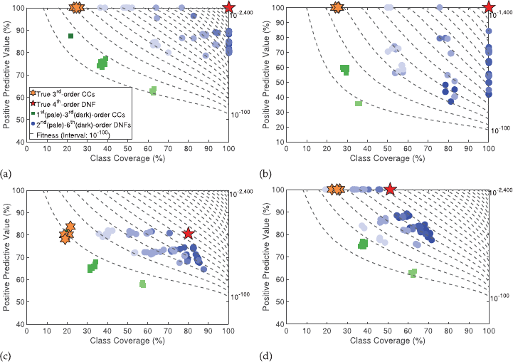
J. P. Hanley et al.
Figure 2: Typical archived results (arbitrarily selected as the rst of 30 repetitions) using
8,000 random training instances for target class 1 on the 6-bit multiplexer problem with
14 extraneous features added and (a) balanced classes with no noise or missing data;
or with either (b) imbalanced class outcomes (15% class 1); (c) 20% random errors in
class outcome; or (d) 20% randomly missing feature data. The contour lines represent
equally spaced values of Fitness.
stands out as the archived DNF with the best Fitness (e.g., Fig. 2c). Finally, we observed
that even with 20% missing data in the input dataset, the true causal DNF always had
orders of magnitude better tness than any other 4th-order DNF (e.g., Fig. 2d), although
in some runs there were a few (median = 7 over the 30 repetitions) 5th and 6th order
clauses that had slightly better tness. In these cases, the true causal DNF could still be
identied as the most parsimonious (i.e., lowest order) of the highly t DNFs.
4.3 Results on Synthetic Genome Problem
The synthetic genome problem includes extraneous features and noise in class out-
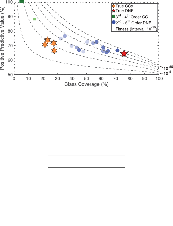
comes, so it is not possible to achieve 100% PPV or coverage. However, all 4 true causal
2nd-order CCs were consistently archived in all 30 repetitions. The true causal 4th-order
DNF was also archived in all 30 trials. We found numerous DNFs with higher PPV than
the true causal DNF and a few other higher-order DNFs with similar or slightly bet-
ter Fitness; however, the true causal DNF stands out as the most parsimonious (lowest
order) of the ttest DNFs in the archive, and as the archived DNF with the highest cov-
erage (see Figure 3).
The synthetic genome problem highlights the importance of using the feature sen-
sitivity test to lter the number of CCs added to the CCEA archive. There are 20 features
in the synthetic genome problem, and only 4 are contained in the true causal rule set.
104
Evolutionary Computation Volume 28, Number 1
A Tandem EA for Identifying Causal Rules
Figure 3: Archived results on the Synthetic Genome Problem (arbitrarily selected as the
rst of 30 repetitions) using the 1,600 training instances. The contour lines represent
equally spaced values of Fitness.
Table 8: Summary of results on the synthetic genome problem. All values are the me-
dian over 30 repetitions. The feature sensitivity test was used in the CCEA for all runs.
Rows are the same as in Table 5.
Synthetic Genome Medians
CCEA Space 1.1 × 10
12
#CCEA Evals 3,529
#Archived CCs 7
DNFEA Space 119
#DNFEA Evals 106
#Archived DNFs 40
#Total Evals 3,595
De novo DNF Space 2.5 × 10
69
Nonetheless, there are thousands of potential CCs that pass the initial ratio and tness
threshold tests for the archive. However, there are only 11 possible CCs that would also
pass the feature sensitivity test. In practice, adding the feature sensitivity lter reduced
the median number of archived CCs to 7 (see Table 8). With so few CCs archived, the
DNFEA required only slightly fewer tness evaluations than exhaustive search (com-
pare the #DNFEA Evals to the size of the DNFEA Space in Table 8).
4.4 Results on Chagas Vector Infestation Dataset
The CCEAarchived 1,089 CCs (Fig. 4), and discovered several interesting heterogeneous
and overlapping CCs (ranging from main effects through 7th-order epistatic CCs). On
this real-world problem, incorporating the feature sensitivity threshold reduced the
maximum order of archived clauses from 24th-order to 7th-order, thus removing thou-
sands of the very high order CCs most likely the product of overtting.
The DNFEA archived 940 probabilistically-signicant DNFs (see Figure 4). In
this real-world dataset, it is unlikely that a single causal DNF exists. Due to feature
Evolutionary Computation Volume 28, Number 1 105
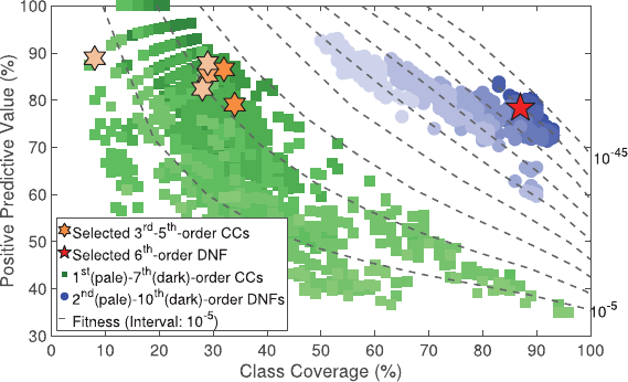
J. P. Hanley et al.
Figure 4: Archived Chagas survey results. Axes represent the PPV and class coverage
on the 311 training instances, 100 of which are associated with infestation. Contours
represent equally spaced Fitness. The pentagram and hexagrams are selected candidates
for possibly causal rule sets.
correlations, missing and noisy data, there are many rule sets with very strong statis-
tical associations with infestation of the Chagas vector. We are also well aware of the
risk of overtting in this relatively small dataset; so we do not claim to have “solved”
the problem. Figure (4) highlights one of many interesting candidate DNFs, selected as
the most parsimonious of the highly t DNFs with Fitness < 10
−39
. This 6th-order DNF
has Fitness = 4 × 10
−40
, PPV = 78%, Coverage = 87%, and comprises CCs ranging from
order 3 to order 5 (also highlighted in Fig. 4), whose coverage sums to 152%, indicating
overlap. This and other highly t DNFs are interesting candidates solutions that may
provide insight into the primary drivers of T. dimidiata infestation.
5 Discussion
To tackle the challenge of seeking potentially causal rules sets for explaining complex
real-world data, we propose a new approach using tandem age-layered evolutionary
algorithms on batch data. In this section, we discuss some key aspects of the CCEA-
DNFEA algorithm, compare our results on benchmark problems to published LCS re-
sults, and briey discuss the application of the method to a real-world survey problem.
5.1 Hypergeometric PMF as a Fitness Metric
We propose using the hypergeometric PMF (Eq. (1)) as a principled statistic rooted in
probability theory (Kendall, 1952) for assessing relative tness of clauses of a given or-
der in complex classication problems. Unlike other tness functions that incorporate
ad hoc weighted sums and/or products of PPV, coverage, and/or model complexity
(Aguilar-Ruiz et al., 2003; Llorà et al., 2008; Bacardit et al., 2009), the hypergeometric
PMF quanties the probability that the observed association between a given clause
and target class is due to chance, taking into account the size of the dataset, the amount
of missing data, and the distribution of outcome categories.
106
Evolutionary Computation Volume 28, Number 1
A Tandem EA for Identifying Causal Rules
We use dynamically-adjusted, order-specic, probability thresholds to determine
which CC and DNF clauses to archive. Of course, while these clauses are potentially
causal, a low probability that the association is by chance does not in itself imply causa-
tion (Nuzzo, 2014). Equation (1) enables our algorithm to archive parsimonious clauses
with different combinations of PPV and coverage while gracefully handling imbalanced
classes, missing data, and noisy class associations.
5.2 CCEA and DNFEA
The CCEAcreates an archive of CCs, each with a probabilistically signicant association
with a given outcome class. The DNFEA subsequently creates an archive of probabilis-
tically signicant disjunctions of the archived CCs. As in Hornby (2006), we found the
age-layering to be very important in maintaining diversity, which facilitated continual
improvement over the evolutionary process.
By maintaining separate archive bins for clauses of different orders, and using a
feature sensitivity threshold to lter the CCs with unwarranted complexity, the tandem
algorithm evolves parsimonious rule sets without aprioriassumptions on the maximum
order of interactions (as in Urbanowicz and Moore, 2015) or the inclusion of ad hoc
penalty terms in the tness function (as in Llorà et al., 2008 and Bacardit et al., 2009).
It is important to note that the CCEA and DNFEA algorithms do not necessarily
need to be run in tandem, and can each be used independently. For example, Hanley
(2017) uses the CCEA alone to mine the Chagas dataset to nd a variety of very t
CCs that could be more closely examined by domain experts to assess (a) new insights
regarding combinations of risk factors associated with T. dimidiata infestation, and (b)
whether these CCs might inform the design of new ecohealth interventions to slow the
spread of Chagas disease in a feasible, effective, and cost-effective manner. Similarly,
the DNFEA can be used independently of the CCEA (e.g., to identify heterogeneous
rule sets comprised of CCs using methods other than the CCEA, such as through LCS,
Genetic Programming, Random Chemistry (Eppstein et al., 2007), or even exhaustive
search (if the size of the CC search space is small enough). Conversely, if the CCEA
archives only a few CCs (as in the synthetic genome problem), one could bypass the
DNFEA and simply use exhaustive search on the CCEA archive to identify the causal
DNF.
5.3 Majority-On Problem: LCS versus CCEA-DNFEA
The presence of overlapping CCs is the primary reason the majority-on problem has
been used as a benchmark in the LCS community (Iqbal et al., 2013b,c, 2014). One of the
most reliable Michigan-style LCSs, referred to as XCS, is known to struggle with overlap
(Kovacs, 2002; Ioannides et al., 2011). Kovacs (2002) noted that XCS penalizes against
overlapping CCs; and Ioannides et al. (2011) showed that even when XCS is initialized
with a population containing the overlapping true signals, they are selected out of the
CC population.
When Iqbal et al. (2013c) used XCS to tackle the 7-bit majority-on problem, the
evolved CCs were an order or two below that of the true causal CCs. On the other
hand, when an XCS variant was used, one that evolves a logical representation of the
action set, the selected CCs were often (23 out of 30 times) at least one order greater than
the true causal CCs (Iqbal et al., 2013c). Thus, even when 100% PPV was reported for
small majority-on problems (3-, 5-, and 7-bit) (Iqbal et al., 2013b,c, 2014), the true causal
CCs were not identied. This is not surprising, given that our analysis (see Fig. B1)
shows many suboptimal CCs with 100% PPV. Signicant overtting is likely in these
Evolutionary Computation Volume 28, Number 1 107
J. P. Hanley et al.
large populations of overly specic classiers. Although total evaluations are not ex-
plicitly reported in the LCS community, we observe from published plots that reported
evaluations for low-order majority-on problems (Iqbal et al., 2013c, 2014) are orders of
magnitude larger than the number of possible CCs in the search space.
In contrast, the proposed CCEA consistently and efciently archived all of the true
causal CCs in all majority-on problems tested (up to 11-bit). The DNFEA archived the
single true causal DNF in up to 5-bit majority-on problems, and this causal DNF was
easily identiable as the archived clause with the best Fitness. Because the feature sensi-
tivity test cannot be employed for the majority-on problem (see Subsection 3.1), ad hoc
postprocessing was required to reduce the size of the CC archive before the DNFEA
could be effectively used for 7-bit to 11-bit majority-on problems.
5.4 Multiplexer Problem: LCS versus CCEA-DNFEA
The presence of tunable degrees of heterogeneity and epistasis is the primary reason
the multiplexer problem continues as a standard benchmark problem in the LCS com-
munity. As the size of the multiplexer problem increases, the number of true CCs in the
true causal DNF increases (albeit not as rapidly as in the majority-on problem) and the
individual coverage rapidly decreases (Table 3). As in previous studies (Kovacs, 1998;
Butz et al., 2003), we also found many noncausal CCs with the same PPV and expected
coverage as the true causal CCs.
Both Michigan-style and Pittsburgh-style LCSs have been used to tackle the multi-
plexer problem. Although the lowest number of training instances used by Michigan-
style LCS on the multiplexer problem shown by Iqbal et al. (2013c, 2014) were the same
order of magnitude as the number of #Total Evals reported here, this LCS was not able
to directly evolve the true causal CCs even when achieving 100% prediction accuracy.
However, with additional ad hoc post-processing, the true causal DNFs were recov-
ered on balanced multiplexer problems up to 37-bits (Iqbal et al., 2013a). Bacardit and
Krasnogor (2009) evolved a nearly-causal rule set for the 37-bit multiplexer problems
using a modied Pittsburgh-style LCS with smart crossover (rst introduced in Bacardit
and Krasnogor, 2006), again using the same order of magnitude number of training in-
stances as #Total Evals reported here; they report that the causal DNF was identied
when the algorithm was allowed to run longer, but did not specify how much longer.
Our proposed approach consistently evolved the single true causal DNF in all mul-
tiplexer problems tested (up to 37-bit). Even when we introduced extraneous features,
imbalanced classes, noise in the class associations, and missing data into a 6-bit multi-
plexer problem, our methodology reliably evolved and identied the single true causal
4th-order DNF of 3rd-order CCs (Fig. 2). It is encouraging that the CCEA and DNFEA
performed so strongly in the face of signicant class imbalance, noise in class associa-
tions, and missing data, because these are often characteristics of real-world datasets.
Of particular importance is the ability to handle missing data, without the need impute
with potentially misleading synthetic data.
5.5 Synthetic Genome Problem: LCS versus CCEA-DNFEA
The synthetic genome problem introduced in Urbanowicz and Moore (2010a) was de-
signed as a more realistic dataset representing a heterogeneous, purely epistatic prob-
lem, in which the true causal DNF is a 4th-order disjunction of four 2nd-order CCs. This
dataset includes 16 extraneous features and an imperfect association between the true
features and balanced binary outcome classes.
108
Evolutionary Computation Volume 28, Number 1
A Tandem EA for Identifying Causal Rules
Urbanowicz and Moore (2010b) report an inability to evolve correct rule sets for
this problem when using a Pittsburgh-style LCS. They used the Michigan-style XCS to
evolve rules for predicting both class 0 and class 1 (Urbanowicz and Moore, 2010a) and
reported an average classication accuracy of over 88% using 10-fold cross validation
with 1,600 classiers trained on 1,440 unique training instances (repeatedly sampled
for a total of 1,000,000 instances shown to XCS), and up to 72% on the testing data.
Thus, despite their use of cross-validation there was still evidence of overtting, since
the average training accuracy was over 20% higher, and the average testing accuracy
over 5% higher, than the accuracy of the true causal rule set.
Our approach consistently archived all 4 true causal CCs and the single true causal
DNF, which was readily identiable as (a) the most parsimonious of the highly t
clauses and (b) had the highest coverage in the resulting DNF archive. This more realis-
tic problem, relative to the majority-on or multiplexer problems, also highlights the im-
portance of using the feature sensitivity test, which reduced the number of CCs passed
to the archive by two orders of magnitude.
5.6 Chagas Vector Infestation Dataset
Some of the feature interactions evolved by the CCEA on the Chagas vector infestation
data had been previously identied as potential drivers of infestation, which increases
our condence in the CCEA results. However, the CCEA analysis also provided ranges
of co-evolved values of interacting features that were most strongly associated with in-
festation as well as new feature interactions not recognized previously. Ongoing anal-
ysis of the CCEA and DNFEA Chagas survey results is being used to inform the design
of eco-interventions aimed at slowing the spread of Chagas disease. While a full discus-
sion of this application is beyond the scope of this article, we refer the interested reader
to Hanley (2017) for more details.
6 Summary
We developed a new method, and provide open source code (Hanley, 2019), for iden-
tifying parsimonious complex rule sets from batch data that may include features of
arbitrary arity and multiple class outcomes.
We use a hypergeometric probability mass function as a principled statistic for as-
sessing tness of potential causal rules in complex classication problems. This tness
function formally quanties the probability that an observed association between a rule
and a class outcome is due to chance, taking into account the size of the dataset, the
amount of missing data, and the distribution of class outcomes. We employ this t-
ness metric in two back-to-back age-layered evolutionary algorithms. The rst evolves
an archive of probabilistically signicant conjunctive clauses, incorporating co-evolved
sets of feature values in these clauses. The second evolves an archive of probabilisti-
cally signicant disjunctions of the archived conjunctions. Each archive uses separate
bins for clauses of different orders, with dynamically adjusted, order-specic tness and
optional feature sensitivity thresholds. The combination of these algorithmic attributes
enables our method to discover parsimonious, epistatic, heterogeneous, and overlap-
ping rule sets, even in the presence of imbalanced classes, missing data, and noisy class
associations.
By decomposing the problem into rst nding good conjunctive clauses and then
nding good disjunctions of them, our approach is shown to dramatically reduce the
size of the search space (relative to alternative methods that seek to evolve compact
rule sets, such as Pittsburgh-style LCSs) and yet returns ”white box,” potentially causal,
Evolutionary Computation Volume 28, Number 1 109
J. P. Hanley et al.
parsimonious rule sets (in contrast to Michigan Style LCSs, which return large popula-
tions of rules, are prone to overtting, and may not even contain the true causal rules).
We validated the method on two types of scalable benchmark problems with known
causal rule sets (majority-on and multiplexer problems, which include various degrees
of heterogeneity, epistasis, and overlap in the rule sets) from datasets where we had
introduced extraneous features, class imbalance, noise in class outcomes, and missing
data. We also validated on a more realistic noisy synthetic genome problem with purely
epistatic and heterogeneous rules. Analyses of the tness landscapes of these problems
illustrate why more ad hoc combinations of PPV and coverage may be insufcient for
identifying the true causal rule sets.
In all the epistatic and heterogeneous benchmark problems tested, we consistently
evolved the true causal rule sets in the form of a single clause in disjunctive normal form,
thus truly solving these problems in the strongest sense of the word. This distinguishes
our method from machine learning classiers whose aim is only to maximize prediction
accuracy and coverage on sampled data. To our knowledge, no other method has been
shown to consistently identify such complex causal rule sets from datasets with this
level of complexity.
Finally, we applied the method to the real-world survey dataset that initially moti-
vated us to develop the method. Our ongoing analysis of the results is providing impor-
tant practical insights to inform eco-intervention strategies aimed at slowing the spread
of the deadly Chagas disease.
Acknowledgments
This work was supported, in part, by Vermont EPSCoR with funds from the National
Science Foundation Grant EEID BCS-1216193 (JPH) and EPS-1101317 (DMR).
References
Aguilar-Ruiz, J., Riquelme, J., and Toro, M. (2003). Evolutionary learning of hierarchical deci-
sion rules. IEEE Transactions on Systems, Man and Cybernetics, Part B (Cybernetics), 33(2):324–
331.
Bacardit, J., Burke, E. K., and Krasnogor, N. (2009). Improving the scalability of rule-based evolu-
tionary learning. Memetic Computing, 1(1):55–67.
Bacardit, J., and Krasnogor, N. (2006). Smart crossover operator with multiple parents for a Pitts-
burgh learning classier system. In Proceedings of the 8th Annual Conference on Genetic and
Evolutionary Computation (GECCO), p. 1441.
Bacardit, J., and Krasnogor, N. (2009). Performance and efciency of memetic Pittsburgh learning
classier systems. Evolutionary Computation, 17(3):307–342.
Barto, A. G. (1985). Learning by statistical cooperation of self-interested neuron-like computing
elements. Human Neurobiology, 4(4):229–256.
Booker, L. B. (1989). Triggered rule discovery in classier systems. In Proceedings of the Third In-
ternational Conference on Genetic Algorithms, Vol. 3, pp. 265–274.
Breiman, L. (2001). Random forests. Machine Learning, 45(1):5–32.
Bustamante Zamora, D. M., Hernández, M. M., Torres, N., Zúniga, C., Sosa, W., de Abrego, V., and
Monroy Escobar, M. C. (2015). Information to act: Household characteristics are predictors of
domestic infestation with the Chagas vector Triatoma dimidiata in Central America. American
Journal of Tropical Medicine and Hygiene, 93(1):97–107.
110 Evolutionary Computation Volume 28, Number 1
A Tandem EA for Identifying Causal Rules
Butz, M., Kovacs, T., Lanzi, P., and Wilson, S. (2004). Toward a theory of generalization and learn-
ing in XCS. IEEE Transactions on Evolutionary Computation, 8(1):28–46.
Butz, M. V., Goldberg, D. E., and Tharakunnel, K. (2003). Analysis and improvement of tness
exploitation in XCS: Bounding models, tournament selection, and bilateral accuracy. Evolu-
tionary Computation, 11(3):239–277.
Butz, M. V., Pelikan, M., Llorà, X., and Goldberg, D. E. (2006). Automated global structure extrac-
tion for effective local building block processing in XCS. Evolutionary Computation, 14(3):345–
380.
Butz, M. V., Sastry, K., and Goldberg, D. E. (2005). Strong, stable, and reliable tness pressure in
XCS due to tournament selection. Genetic Programming and Evolvable Machines, 6(1):53–77.
Buxbaum, J. D., Silverman, J. M., Smith, C. J., Kilifarski, M., Reichert, J., Hollander, E., Lawlor,
B. A., Fitzgerald, M., Greenberg, D. A., and Davis, K. L. (2001). Evidence for a susceptibility
gene for autism on chromosome 2 and for genetic heterogeneity. The American Journal of
Human Genetics, 68(6):1514–1520.
Calian, D. A., and Bacardit, J. (2013). Integrating memetic search into the BioHEL evolutionary
learning system for large-scale datasets. Memetic Computing, 5(2):95–130.
De Jong, K. A., and Spears, W. M. (1991). Learning concept classication rules using genetic algo-
rithms. In Proceedings of the Twelfth International Joint Conference on Articial Intelligence, Vol.
12, pp. 651–656.
Eppstein, M. J., and Hines, P. D. H. (2012). A “random chemistry” algorithm for identifying col-
lections of multiple contingencies that initiate cascading failure. IEEE Transactions on Power
Systems, 27(3):1698–1705.
Eppstein, M. J., Payne, J. L., White, B. C., and Moore, J. H. (2007). Genomic mining for complex
disease traits with random chemistry. Genetic Programming and Evolvable Machines, 8(4):395–
411.
Franco, M. A., Krasnogor, N., and Bacardit, J. (2011). Modelling the initialisation stage of the
ALKR representation for discrete domains and GABIL encoding. In Proceedings of the 13th
Annual Conference on Genetic and Evolutionary Computation (GECCO), pp. 1291–1298.
Franco, M. A., Krasnogor, N., and Bacardit, J. (2012). Analysing BioHEL using challenging
Boolean functions. Evolutionary Intelligence, 5(2):87–102.
Goldberg, D. E. (1989). Genetic algorithms in search, optimization, and machine learning.Reading,MA:
Addison-Wesley.
Hanley, J. P. (2017). A new evolutionary algorithm for mining noisy, epistatic, geospatial survey
data associated with Chagas disease. PhD thesis, Faculty of the Graduate College, The Uni-
versity of Vermont.
Hanley, J. P. (2019). MATLAB code available at https://www.mathworks.com/matlabcentral
/leexchange/69950-ccea-and-dnfea.
Hanley, J. P., Eppstein, M. J., Buzas, J. S., and Rizzo, D. M. (2016). Evolving probabilistically sig-
nicant epistatic classication rules for heterogeneous big datasets. In Proceedings of the 18th
Annual Conference on Genetic and Evolutionary Computation, pp. 445–452.
Holland, J. H., and Reitman, J. S. (1978). Cognitive systems based on adaptive algorithms. In An
overview of pattern-directed inference systems, pp. 313–329. Rand Corporation, Santa Monica,
CA.
Hornby, G. S. (2006). ALPS: The age-layered population structure for reducing the problem of
premature convergence. In Proceedings of the 8th Annual Conference on Genetic and Evolutionary
Computation, p. 815.
Evolutionary Computation Volume 28, Number 1 111
J. P. Hanley et al.
Huang, G. Q., Li, L., and Chen, X. (2007). A tandem evolutionary algorithm for platform product
customization. Journal of Computing and Information Science in Engineering, 7(2):151–159.
Ioannides, C., Barrett, G., and Eder, K. (2011). XCS cannot learn all Boolean functions. In Proceed-
ings of the 13th Annual Conference on Genetic and Evolutionary Computation, p. 1283.
Iqbal, M., Browne, W. N., and Mengjie Zhang (2014). Reusing building blocks of extracted knowl-
edge to solve complex, large-scale Boolean problems. IEEE Transactions on Evolutionary Com-
putation, 18(4):465–480.
Iqbal, M., Browne, W. N., and Zhang, M. (2012). Extracting and using building blocks of knowl-
edge in learning classier systems. In Proceedings of the 14th Annual Conference on Genetic and
Evolutionary Computation, p. 863.
Iqbal, M., Browne, W. N., and Zhang, M. (2013a). Evolving optimum populations with XCS clas-
sier systems: XCS with code fragmented action. Soft Computing, 17(3):503–518.
Iqbal, M., Browne, W. N., and Zhang, M. (2013b). Extending learning classier system with cyclic
graphs for scalability on complex, large-scale Boolean problems. In Proceedings of the 15th
Annual Conference on Genetic and Evolutionary Computation, p. 1045.
Iqbal, M., Browne, W. N., and Zhang, M. (2013c). Learning complex, overlapping and niche imbal-
ance Boolean problems using XCS-based classier systems. Evolutionary Intelligence, 6(2):73–
91.
Iqbal, M., Browne, W. N., and Zhang, M. (2015). Improving genetic search in XCS-based clas-
sier systems through understanding the evolvability of classier rules. Soft Computing,
19(7):1863–1880.
Jarlenski, M., Hyon Baik, S., and Zhang, Y. (2016). Trends in use of medications for smoking ces-
sation in Medicare, 2007–2012. American Journal of Preventive Medicine, 51(3):301–308.
Kaplinski, M., Jois, M., Galdos-Cardenas, G., Rendell, V. R., Shah, V., Do, R. Q., Marcus, R., Bur-
roughs Pena, M. S., del Carmen Abastoor, M., LaFuente, C., Bozo, R., Valencia, E., Ve-
rastegui, M., Colanzi, R., Gilman, R. H., and Bern, C. (2015). Sustained domestic vector ex-
posure is associated with increased Chagas cardiomyopathy risk but decreased parasitemia
and congenital transmission risk among young women in Bolivia. Clinical Infectious Diseases,
61(6):918–926.
Kendall, M. G. (1952). The advanced theory of statistics, volume 1. 3rd ed. New York: Hafner Pub-
lishing Company.
Kirino, Y., Bertsias, G., Ishigatsubo, Y., Mizuki, N., Tugal-Tutkun, I., Seyahi, E., Ozyazgan, Y.,
Sacli, F. S., Erer, B., Inoko, H., et al. (2013). Genome-wide association analysis identies new
susceptibility loci for Behcet’s disease and epistasis between hla-b [ast] 51 and erap1. Nature
Genetics, 45(2):202–207.
Kovacs, T. (1998). XCS classier system reliably evolves accurate, complete, and minimal rep-
resentations for Boolean functions. In P. K. Chawdhry, R. Roy, and R. K. Pant (Eds.), Soft
computing in engineering design and manufacturing, pp. 59–68. London: Springer London.
Kovacs, T. (2002). What should a classier system learn and how should we measure it? Soft
Computing—A Fusion of Foundations, Methodologies and Applications, 6(3–4):171–182.
Larivière, S. (2001). Ursus americanus. Mammalian Species, 647:1–11.
LeCun, Y., Bengio, Y., and Hinton, G. (2015). Deep learning. Nature, 521(7553):436.
Li, K., Simons-Morton, B., Gee, B., and Hingson, R. (2016). Marijuana-, alcohol-, and drug-
impaired driving among emerging adults: Changes from high school to one-year post-high
school. Journal of Safety Research, 58:15–20.
112 Evolutionary Computation Volume 28, Number 1
A Tandem EA for Identifying Causal Rules
Llorà, X., Sastry, K., and Goldberg, D. (2005). The compact classier system: Scalability analysis
andrstresults.InThe 2005 IEEE Congress on Evolutionary Computation, Vol. 1, pp. 596–603.
Llorà, X., Sastry, K., Lima, C. F., Lobo, F. G., and Goldberg, D. E. (2008). Linkage learning, rule rep-
resentation, and the X-ray extended compact classier system. In 10th International Workshop,
pp. 189–205.
Markellos, R. N., Psychoyios, D., and Schneider, F. (2016). Sovereign debt markets in light of the
shadow economy. European Journal of Operational Research, 252(1):220–231.
McDermott, J., De Jong, K., O’Reilly, U.-M., White, D. R., Luke, S., Manzoni, L., Castelli, M., Van-
neschi, L., Jaskowski, W., Krawiec, K., and Harper, R. (2012). Genetic programming needs
better benchmarks. In Proceedings of the 14th Annual Conference on Genetic and Evolutionary
Computation, p. 791.
Molina, I., Salvador, F., Sánchez-Montalvá, A., Trevi no, B., Serre, N., Sao Avilés, A., and Almi-
rante, B. (2015). Toxic prole of Benznidazole in patients with chronic Chagas disease:
Risk factors and comparison of the product from two different manufacturers. Antimicro-
bial Agents and Chemotherapy, 59(10):6125–6131.
Moore, J. H. (2003). The ubiquitous nature of epistasis in determining susceptibility to common
human diseases. Human Heredity, 56(1–3):73–82.
Nesheli, M. M., Ceder, A. A., and Estines, S. (2016). Public transport user’s perception and deci-
sion assessment using tactic-based guidelines. Transport Policy, 49:125–136.
Nuzzo, R. (2014). Scientic method: Statistical errors. Nature, 506(7487):150–152.
Olivera, M. J., Cucunuba, Z. M., Alvarez, C. A., and Nicholls, R. S. (2015). Safety prole of Nifur-
timox and treatment interruption for chronic Chagas disease in Colombian adults. American
Journal of Tropical Medicine and Hygiene, 93(6):1224–1230.
Poole, K. T., and Rosenthal, H. (1984). The polarization of American politics. The Journal of Politics,
46(4):1061–1079.
Rapp, J. P., Garrett, M. R., and Deng, A. Y. (1998). Construction of a double congenic strain to
prove an epistatic interaction on blood pressure between rat chromosomes 2 and 10. Journal
of Clinical Investigation, 101(8):1591–1595.
Ritchie, M. D., Hahn, L. W., Roodi, N., Bailey, L. R., Dupont, W. D., Parl, F. F., and Moore,
J. H. (2001). Multifactor-dimensionality reduction reveals high-order interactions among
estrogen-metabolism genes in sporadic breast cancer. The American Journal of Human Genetics,
69(1):138–147.
Smith, S. F. (1980). A learning system based on genetic adaptive algorithms. PhD thesis, University
of Pittsburgh.
Urbanowicz, R. J., Andrew, A. S., Karagas, M. R., and Moore, J. H. (2013). Role of genetic het-
erogeneity and epistasis in bladder cancer susceptibility and outcome: A learning classier
system approach. Journal of the American Medical Informatics Association, 20(4):603–612.
Urbanowicz, R. J., Bertasius, G., and Moore, J. (2014). ExSTraCS 1.0: An extended Michigan-style
learning classier system for exible supervised learning. In Parallel Problem Solving from
Nature, pp. 211–221.
Urbanowicz, R. J., and Moore, J. H. (2009). Learning classier systems: A complete introduction,
review, and roadmap. Journal of Articial Evolution and Applications, 2009:1–25.
Urbanowicz, R. J., and Moore, J. H. (2010a). The application of Michigan-style learning classier
systems to address genetic heterogeneity and epistasis in association studies. In Proceedings
of the 12th Annual Conference on Genetic and Evolutionary Computation, p. 195.
Evolutionary Computation Volume 28, Number 1 113
J. P. Hanley et al.
Urbanowicz, R. J., and Moore, J. H. (2010b). The application of Pittsburgh-style learning classier
systems to address genetic heterogeneity and epistasis in association studies. In International
Conference on Parallel Problem Solving from Nature, pp. 404–413.
Urbanowicz, R. J., and Moore, J. H. (2015). ExSTraCS 2.0: Description and evaluation of a scalable
learning classier system. Evolutionary Intelligence, 8(2–3):89–116.
Wilson, I. D. (2009). Drugs, bugs, and personalized medicine: Pharmacometabonomics enters the
ring. Proceedings of the National Academy of Sciences, 106(34):14187–14188.
Wilson, N. L., Rickard, B. J., Saputo, R., and Ho, S.-T. (2017). Food waste: The role of date labels,
package size, and product category. Food Quality and Preference, 55:35–44.
Wilson, S. W. (1987a). Classier systems and the animat problem. Machine Learning, 2(3):199–228.
Wilson, S. W. (1987b). Quasi-Darwinian learning in a classier system. In Proceedings of the Fourth
International Machine Learning Workshop, Vol. 4, pp. 59–65.
Wilson, S. W. (1995). Classier tness based on accuracy. Evolutionary Computation, 3(2):149–175.
Wu, X., Zhu, X., Wu, G.-Q., and Ding, W. (2014). Data mining with big data. IEEE Transactions on
Knowledge and Data Engineering, 26(1):97–107.
Young Kim, E., and Kim, Y. (2004). Predicting online purchase intentions for clothing products.
European Journal of Marketing, 38(7):883–897.
Youse, S., Moradi, H., Boll, J., and Schönbrodt-Stitt, S. (2016). Effects of road construction on soil
degradation and nutrient transport in Caspian Hyrcanian mixed forests. Geoderma, 284:103–
112.
114 Evolutionary Computation Volume 28, Number 1
